As an editor, you likely know a lot more about Microsoft Word than the average person! What you might not know is that Microsoft Excel also has a lot to offer the hard-working editor. In this two-part series, we’ll discuss six ways you can use Excel to make Word work better.

In Part 1, we talked about how to use Excel to work with numbers: checking calculations, reformatting numbers, and converting from one measurement system to another. In Part 2, we’ll explore some surprising ways Excel can help you wrangle text!

This is an interactive blog post! Instead of using screenshots of the Word content we’re working with, we’ve used text and tables you can copy and paste.

But I thought Excel was for budgets!

In addition to helping you manage budgets, keep track of production schedules, and double-check your math, Excel can help you with a whole range of tasks related to managing lists and tables, including

• Sorting list items alphabetically, chronologically, or numerically
• Sophisticated multi-column sorting that Word can’t handle
• Dividing one column of text into two or more columns
• Merging two or more columns of text together
• Removing duplicates from a list or a table
• Turning a list or other delimited text into a table

Sorting lists

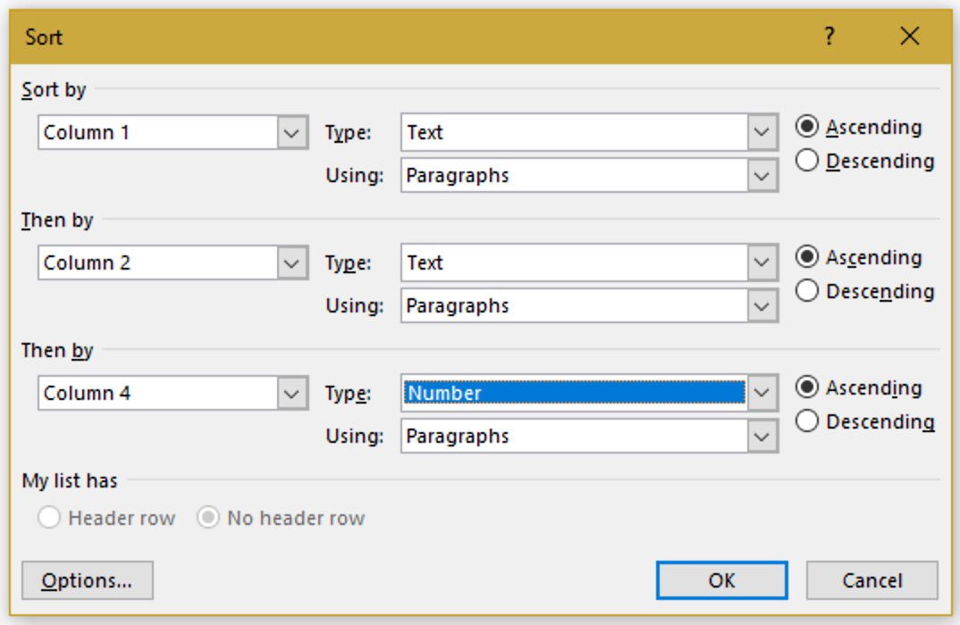
Word’s Sort button lets you sort selected text (usually a list or a table column) in alphabetical, numerical, or chronological order. This is great as far as it goes—but Word only allows three sorting parameters:

If you need more than that, Excel is your friend!

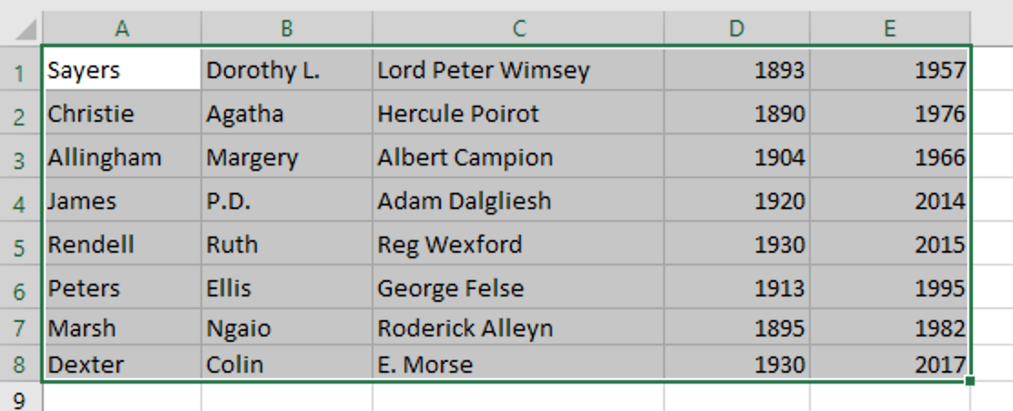
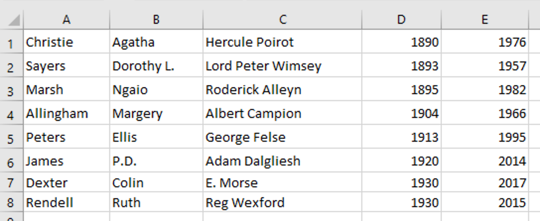
For example, imagine you wanted to sort this table chronologically by year of birth, then alphabetically by surname and given name, then chronologically by year of death. (And since this is a very simple table created to illustrate this blog post, imagine the much longer, wider, and more complex table you’re more likely to see in reality!)

 

Sayers	Dorothy L.	Lord Peter Wimsey	1893	1957
Christie	Agatha	Hercule Poirot	1890	1976
Allingham	Margery	Albert Campion	1904	1966
James	P.D.	Adam Dalgliesh	1920	2014
Rendell	Ruth	Reg Wexford	1930	2015
Peters	Ellis	George Felse	1913	1995
Marsh	Ngaio	Roderick Alleyn	1895	1982
Dexter	Colin	E. Morse	1930	2017

 

To work with the text in Excel, start by selecting the whole table, copying it, and pasting it into a new Excel sheet.

→ Tip: In a new, empty Excel sheet, you can simply position your cursor or mouse pointer in any cell and paste; the contents will spread themselves out appropriately. To follow along with this example, use cell A1 (the top left-hand cell).

Next, make sure everything you just pasted is still selected:

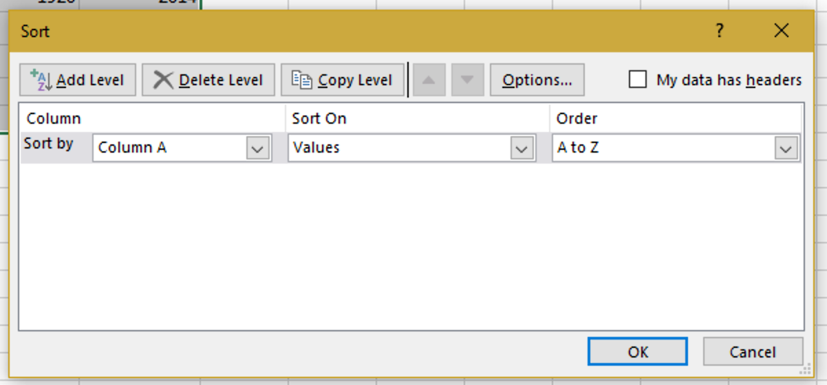
And click Home > Sort & Filter > Custom Sort to bring up the Custom Sort dialog:

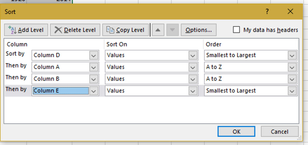
Excel lets you add as many levels as there are columns. For this example, we’ll ask Excel to sort column D (birth year) from smallest to largest, columns A and B from A to Z, and column E (death year) from smallest to largest:

→ Tip: In Excel, just like in Word, if your columns have headers, you should click the My data has headers box to exclude the header row from sorting; this will also change the column names from “Column X” to the header text.

Click OK, and you get this result:

which can be pasted right back into your Word file as a table.

To appreciate how valuable Excel’s more sophisticated sorting capabilities can be, imagine that this table included multiple authors born in the same year, multiple authors with the same surname, and multiple authors who died in the same year.

Splitting text

For Word users, one of Excel’s most useful features is the Text to Columns function.

Suppose you have this list:

which you need to convert into a table like the one above. Excel can help!

→ Tip: You can use the same steps to help you rearrange the list in other ways—such as reversing surnames and given names (Lin-Manuel Miranda → Miranda, Lin-Manuel), changing the date format, removing dates, or removing first names—that are tedious and inefficient to do by hand.

First, select the whole list and paste it into Excel.

→ Tip: In a new, empty Excel sheet, you can simply position your cursor or mouse pointer in any cell and paste; the contents will spread themselves out appropriately. To follow along with this example, use cell A1 (the top left-hand cell).

You should now have something like this:

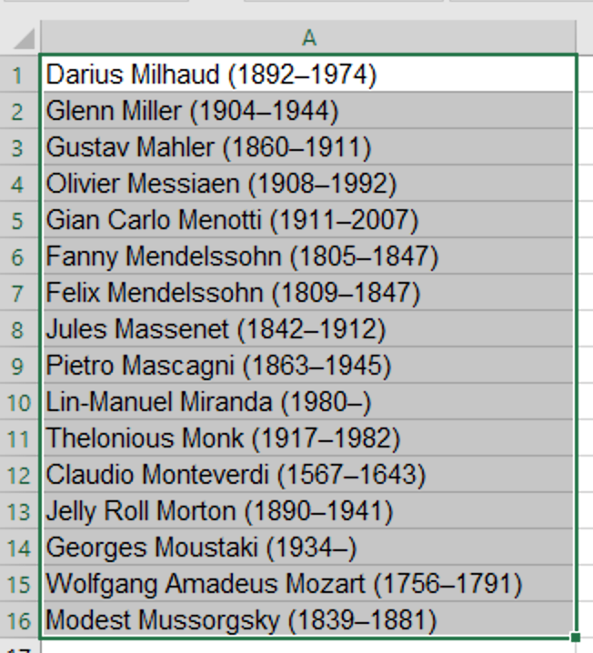
where each list item has its own spreadsheet row, but everything is in the same column.

Next, click Data > Text to Columns to bring up the Text to Columns wizard, and under Original data type, choose Delimited:

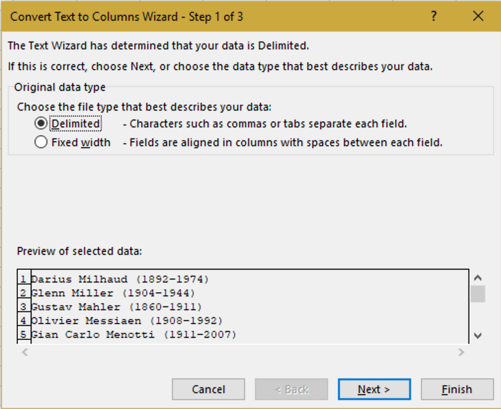
Then click Next.

At this stage, Excel gives you some choices about how to split up your list items:

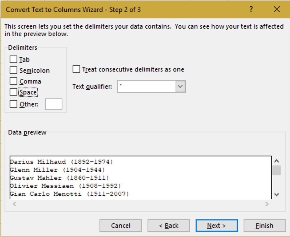
To separate given names from surnames and surnames from dates, we want to check the Space box.

The Text to Columns wizard also helpfully provides a data preview:

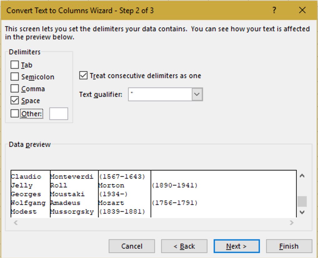
In this case, it tells us that this won’t be a one-step process, because three people on the list (Menotti, Morton, and Mozart) with two-part given names. Pay close attention to the preview window, especially in situations more high-stakes than this example!

In step 3 of the Text to Columns wizard, you can review and change the data type for each column:

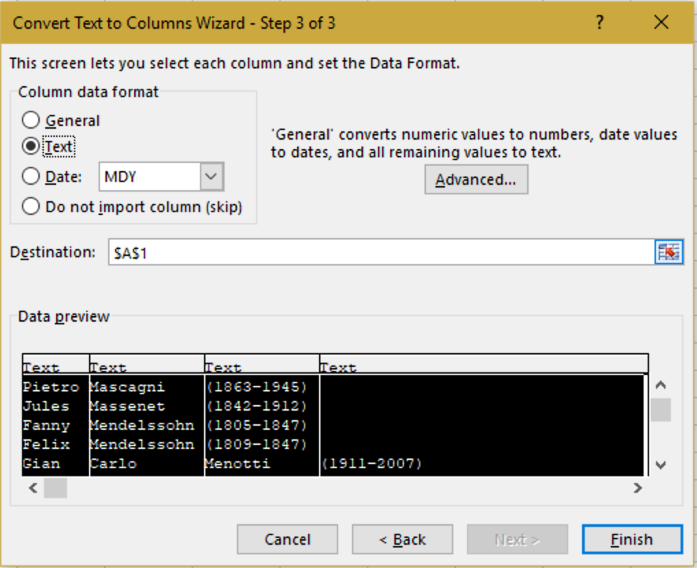
In this case, we’ll make them all Text. (If you make the wrong choice, don’t worry! You can change the data type at any point in Excel.)

Click Finish.

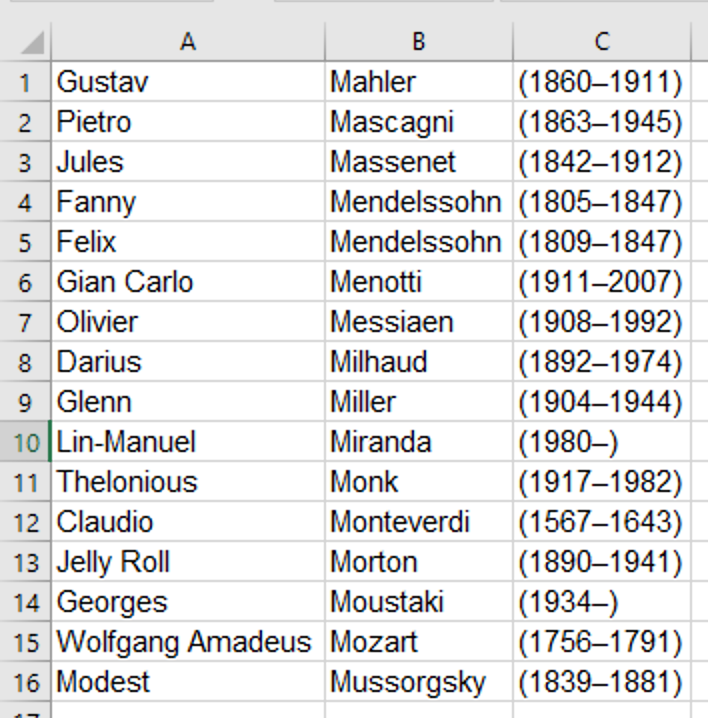
Here’s what you should now see:

And with a very small amount of tidying, you end up with this:

Which you can now copy and paste into Word, ending up with a lovely Word table.

→ Tip: An alternative to post-split tidying is to start by replacing the spaces between, for example, Jelly and Roll with non-breaking spaces. Excel, like Word, reads different types of spaces differently, and you can use this to your advantage!

You could also split apart the birth and death dates, as in our mystery writer example above, using Text to Columns with – as the delimiter, and finish up with two Find and Replace passes that replace ( and ) with nothing.

Joining text

Now suppose that, instead of a table, you wanted to end up with a list in this format:

Mahler, Gustav (1860–1911)

In this case, your first few steps are the same: use Text to Columns to split your list into 3 columns for given name/s, surname, and date/s.

Next, select column A, right-click or use Ctrl-X to cut (you’ll see a dotted line appear around your cut or copied selection), then select column B, right-click, and choose Insert Cut Cells.

You should now have surnames in column A and given names in column B, and it’s time to break out a formula!

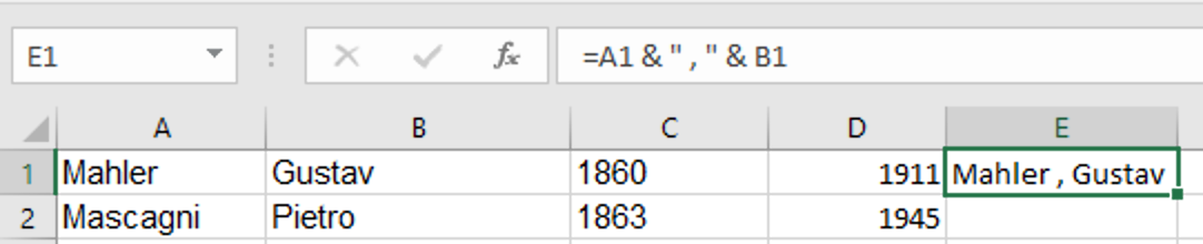
Here’s the basic formula: =A1 & “, ” & B1

You can put it in any blank cell; here we’ve put it in the next available one.

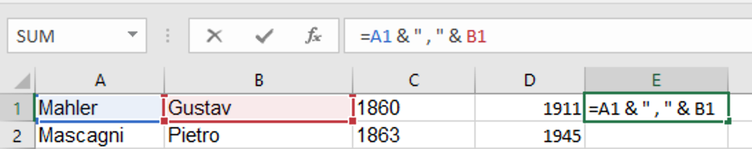
What’s going on here? Basically, we’re borrowing Excel’s ability to add numbers and using it to “add” (concatenate) pieces of text. Cell A1 is the surname, B1 is the given name, and we are asking Excel to add them together (&) and put a comma and a space between them (, ). Anything that isn’t a variable (A1, B1, etc.) or an operator (&, which tells Excel to join two things together) must be enclosed in ” “ to indicate that it’s to be dropped in as is.

As you can see in the screenshot above, Excel helpfully color-codes the content of the formula bar to match the content of the corresponding spreadsheet cells, which makes it easier to see what the formula is going to do.

→ Tip: If your cursor is in the formula bar and you’re not seeing the cell names in different colors, something is wrong with your formula!

Here’s the result:

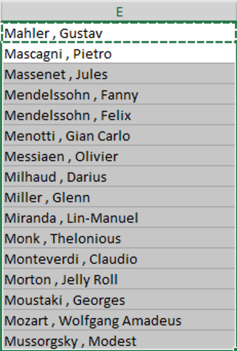
You can then copy the content of cell E1 and paste it into all the cells below it, and you’ll get this:

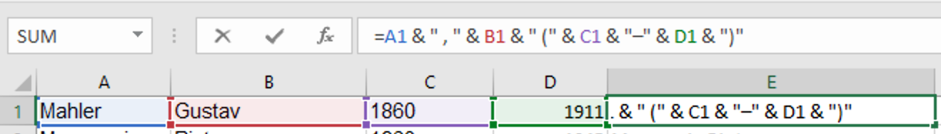
But remember, what we actually want is a list in this format:

Mahler, Gustav (1860–1911)

So our formula will have to get a little more complex: =A1 & “, ” & B1 & ” (” & C1 & “–” & D1 & “)”

Which produces this:

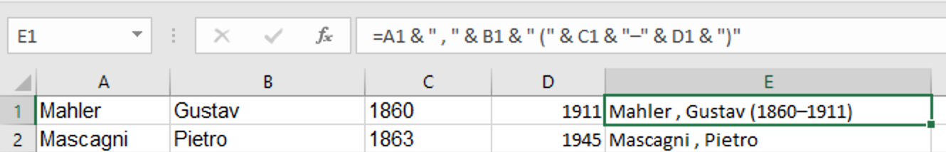
Just copy and paste this cell into all the other cells in column E in order to completely reformat your list:

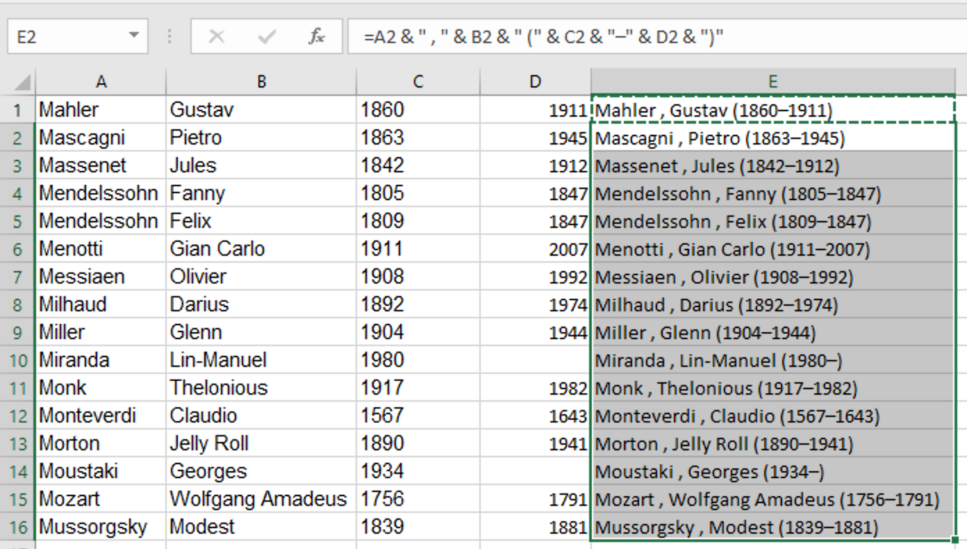
Then, copy and paste cells E1 through E16 into Word:

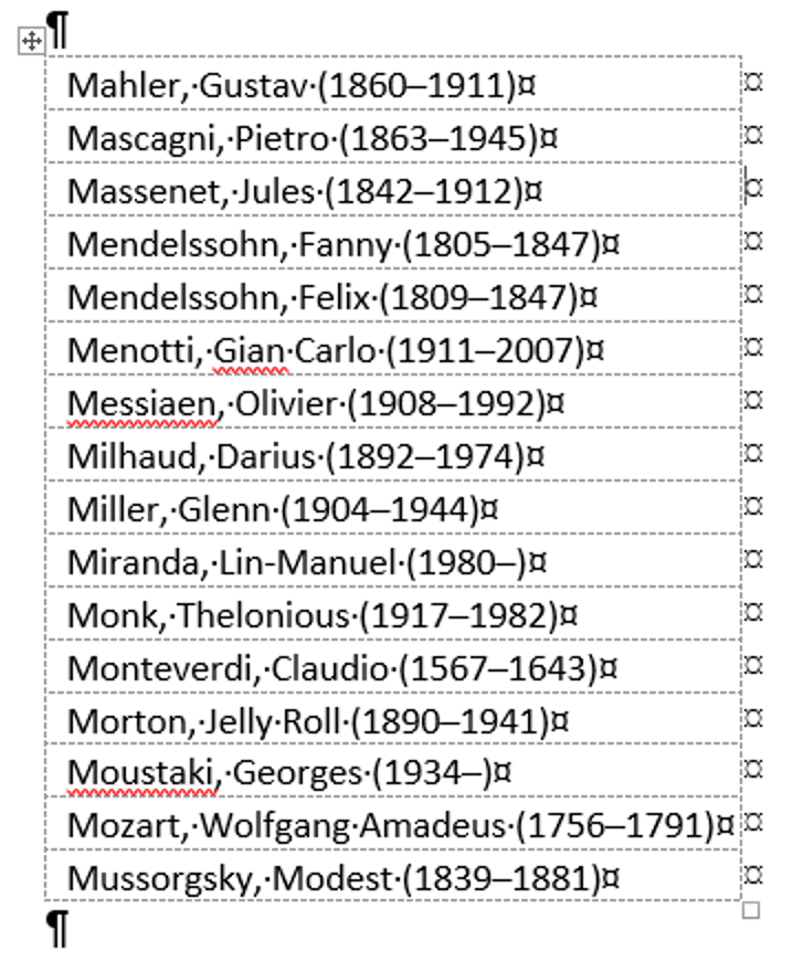
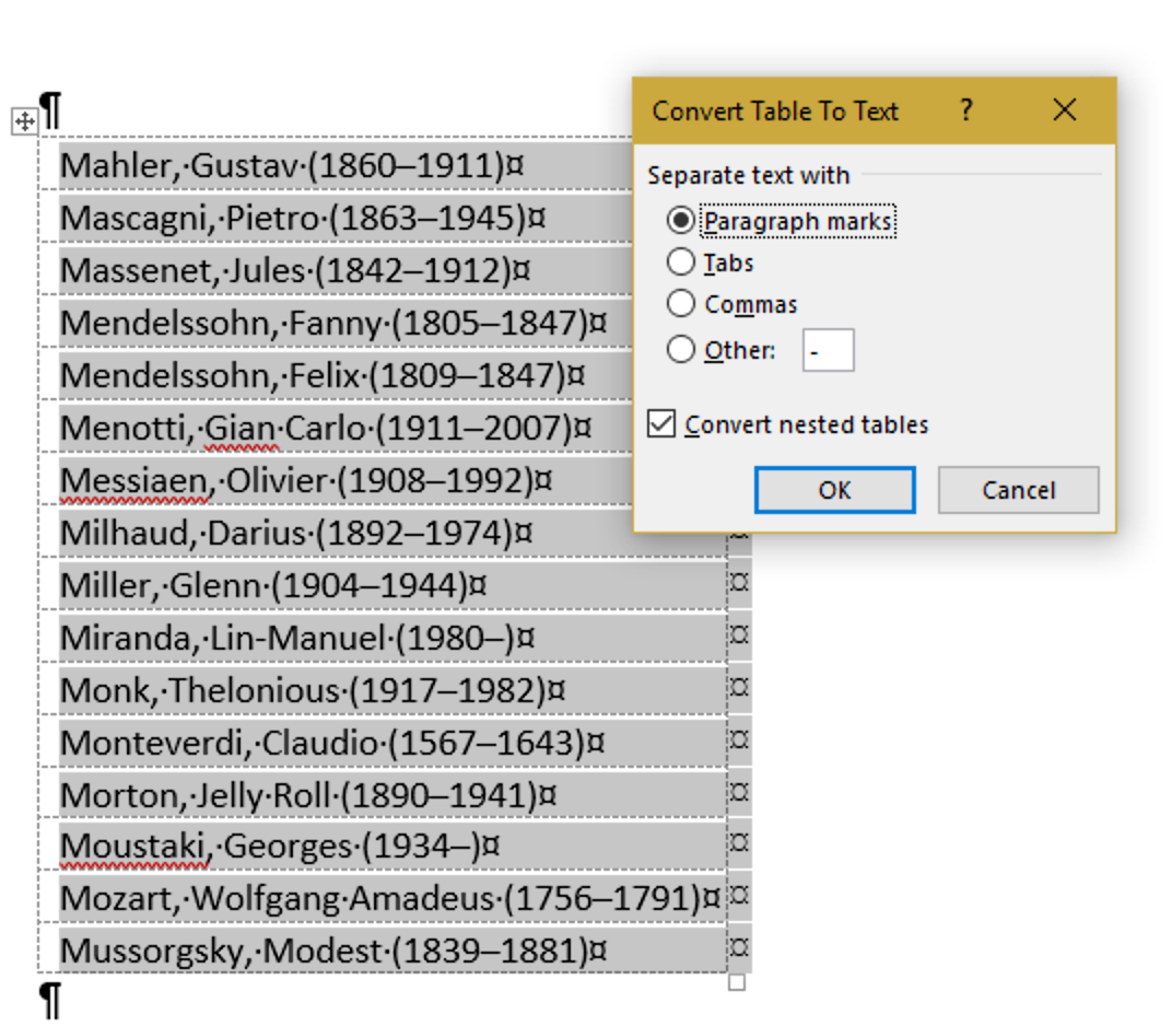
This is still a table, but Word makes it easy to convert a simple table to text: Select the whole table, click Table Tools > Layout > Convert to Text, and under Separate text with, choose Paragraph marks:

Result:

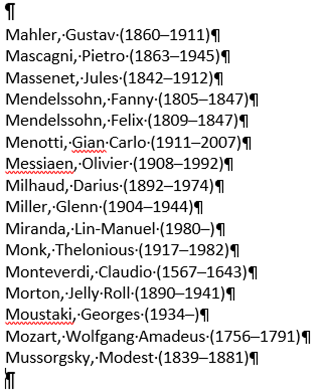
Again, to fully appreciate how much time and effort Excel can save you on tasks like this one, imagine that our list of composers included all 26 letters of the alphabet!