As an editor, you likely know a lot more about Microsoft Word than the average person! What you might not know is that Microsoft Excel also has a lot to offer the hard-working editor. In this two-part series, we’ll discuss six ways you can use Excel to make Word work better.

In Part 1, we’ll talk about how to use Excel to check calculations, reformat numbers, and convert from one measurement system to another.

This is an interactive blog post! Instead of using screenshots of the Word content we’re working with, we’ve used text and tables you can copy and paste.

Checking authors’ math

If you edit in any science or social science field, chances are it’s part of your job to review authors’ calculations and check them for accuracy—in text, in appendices, and especially in tables.

You can perform these checks with a calculator, of course—but you can save a lot of time by handing the job over to Excel! You don’t need expert knowledge to do this; you just need a basic understanding of how Excel’s formulas are organized.

Here’s an example:

	Q1	Q2	Q3	Q4
R1	1.2	26.0	4.4	8.8
R2	3.1	27.1	5.2	27.1
R3	4.5	26.4	11.1	56.2
R4	1.0	28.3	0.2	0.9
Mean	2.5	27.0	5.5	23.3

 

To check the calculations in Excel, follow these steps:

1. Copy the whole table.
2. Open a new Excel file and paste the contents of your clipboard into the file.
   → Tip: In a new, empty Excel sheet, you can simply position your cursor or mouse pointer in any cell and paste; the contents will spread themselves out appropriately. To follow along with this example, use cell A1 (the top left-hand cell).
3. Delete the contents of cells B6 through E6 (the bottom row, excepting the first column).
4. In cell B6, type =average(b2:b5). This will add the four figures above and divide the
   total by 4.
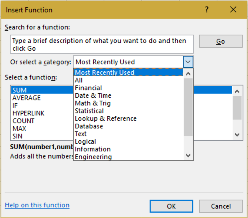
   → Tip: Use the Insert Function button on the Formulas tab to get help with formula structure and explore what functions are available and what they do.

   →

5. Select cell B6, copy, and paste into cells C6, D6, and E6. Excel will automatically adjust the variables to match each row, so that in the formula
   bar you’ll see =average(c2:c5) in column C, and so on.
   → Tip: You can do this one cell at a time, but you can also do it in one step by selecting all 3 cells before hitting Paste!
   → Pro Tip: Save keystrokes with the Home > Fill command! In this case, fill in cells C6, D6, and E6 using Home > Fill > Right (Ctrl-r on the keyboard).
6. Compare the means Excel gives you to those in the author’s table, and query any discrepancies.

If you’ve been following along with this exercise, you’ll have found the error in column D ????

Excel’s library contains hundreds of formulas, many of which you can use in similar ways, including =sum(), =product() and =quotient(); =round(), =ceiling(), =floor(), and other formulas for rounding; =count() and its variations.

Changing number formats

When you need to change how numbers in a table or list align, Word is your best ally. But Excel can help you add, remove, or change currency symbols; increase or decrease decimal places; format times and dates; switch between decimal numbers and fractions; and add leading zeroes when house style calls for them.

The tools you need for all of these actions are found in the Number group on the Home tab:

→

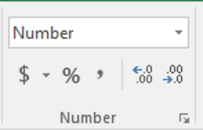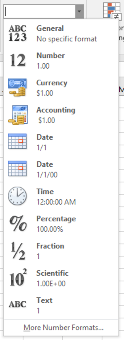Most of these menu choices are self-explanatory; to illustrate, here’s the cell content 0.5 with several different data formats applied:

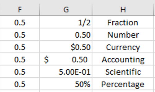
Column G shows the different formats, and in column H we’ve typed their names. “Under the hood,” the content of column G is exactly the same as column F! Copy and paste any of those cells into Word, though, and you’ll get the output (e.g., ½), not the input (0.5).

Converting measures

When house style calls for metric measurements but authors use American ones—or vice versa—Excel has the formula you need.

Just put all your numbers in column A, and in column B, use the formula =convert(). This formula requires 3 inputs, which the formula bar in Excel will prompt you to provide: =convert(number, from_unit, to_unit). Excel will also tell you what short forms to use for pretty much any unit of measure you can think of:

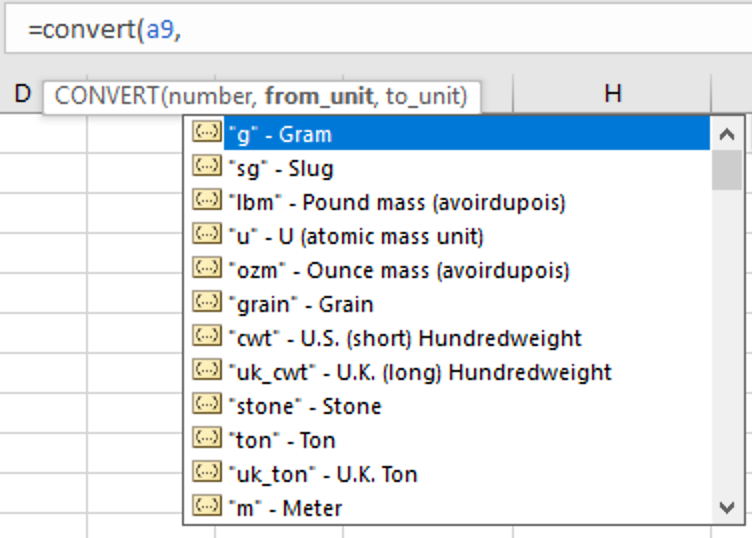
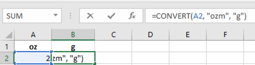
In this example, we’re converting masses from ounces to grams:

→

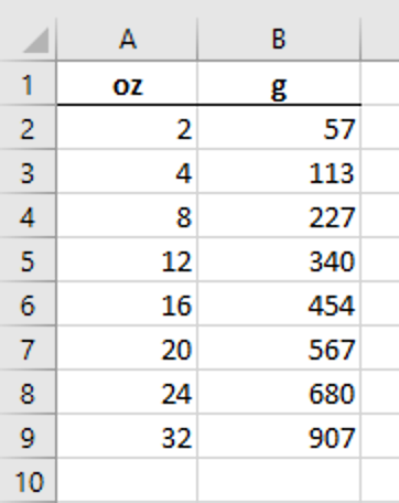→ Tip: You only have to insert the formula once! Then you can copy it into all the other cells where you need it to appear, or use Home > Fill > Down (Ctrl-d on the keyboard). Excel will automatically adjust, changing A2 to A3, A4, and so on.

In Part 2 of this series, we tackle some Excel tips that don’t involve numbers, math, or measurements. Read on!